GRPO From First Principles: Why On-Policy RL for LLMs Is Really Just Dynamic Weighted SFT

Most explanations of PPO, GRPO, and RLHF open the same way: with a wall of formulas. Policy gradients, advantage functions, KL penalties, Monte Carlo estimators, old policies, reference models, clipping terms, reward models. All of it, all at once.

If you already think in reinforcement learning, that’s efficient. If your instincts were shaped by modern supervised training (cross entropy, next-token prediction, SFT, backprop), it’s a brick wall.

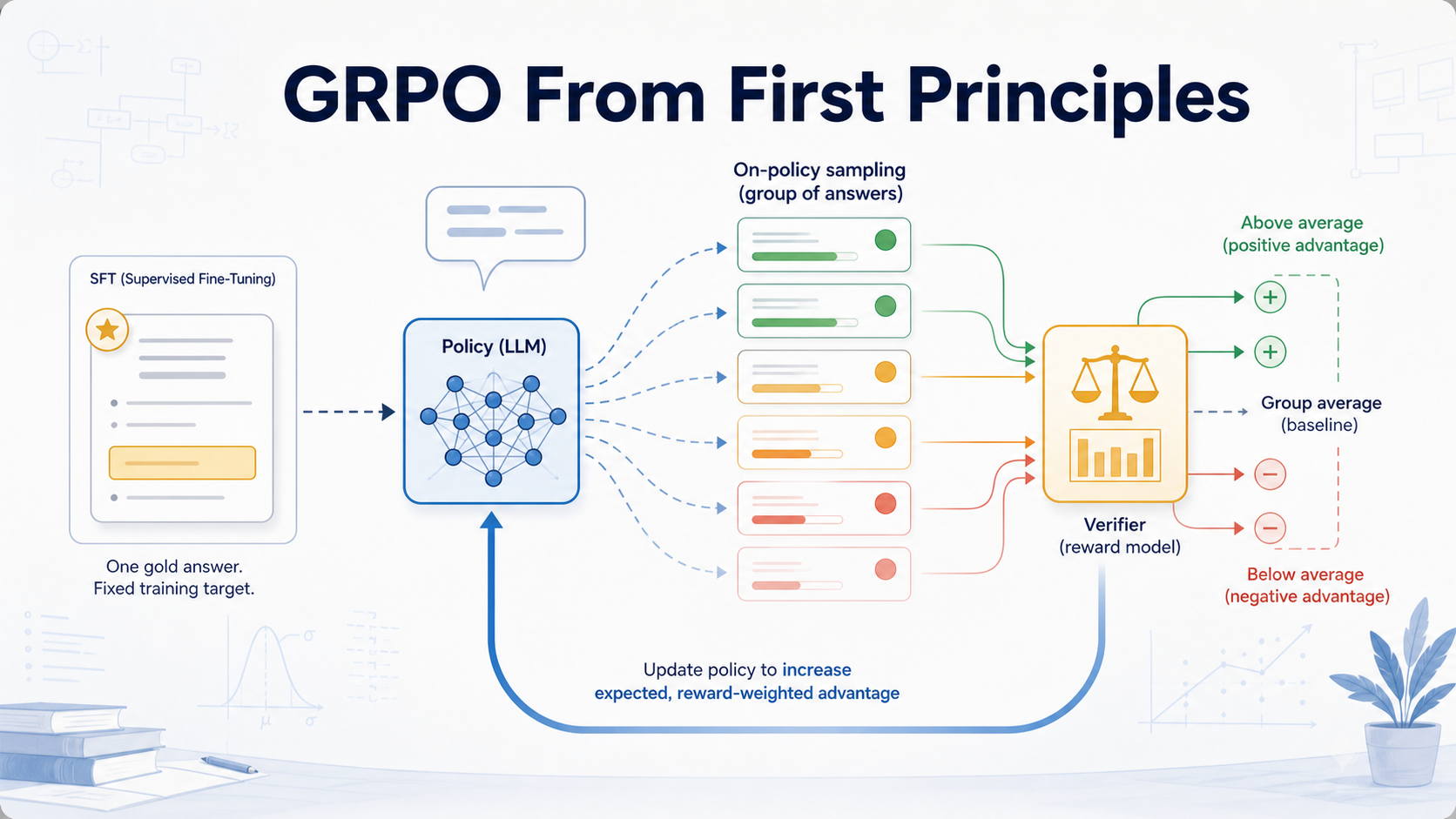
This article takes the other road. We start from the most familiar object in LLM training, supervised fine-tuning, and walk step by step until we arrive at policy gradient and GRPO. The whole journey is organized around one question:

If a model produces an output, and an external verifier scores that output, how do we update the model when the reward itself is not differentiable?

The answer isn’t magic. It’s one of the most useful tricks in all of reinforcement learning:

Don’t try to differentiate through the reward. Instead, raise the probability of outputs that beat a baseline, and lower the probability of outputs that fall short of it.

Once you see it that way, on-policy RL for LLMs stops being mysterious. The whole thing collapses into a single sentence:

GRPO is dynamic, group-normalized, reward-weighted SFT on model-generated samples.

That sentence isn’t the entire story, but it’s the right thing to keep in your head as the story unfolds.

---

Table of Contents

• 1. The Teacher, the Student, and the Missing Answer Key
• 2. Generative AI Is Not Automatically Stochastic
• 3. The Deterministic Strategy and the Gradient Gap
• 4. The Stochastic Strategy: Optimize the Distribution
• 5. SFT First: Increasing the Probability of a Gold Answer
• 6. Why We Need the Log Trick
• 7. Monte Carlo: Engineering the Law of Large Numbers
• 8. From Gradient Estimator to Loss
• 9. GRPO: Group Relative Policy Optimization
• 10. Why KL Regularization Appears
• 11. When Should You Reach for SFT, DPO, PPO, or GRPO?
• 12. Beyond LLMs: Why Probability Matters
• 13. The Whole Picture

---

1. The Teacher, the Student, and the Missing Answer Key

Start in a classroom.

In supervised fine-tuning, the teacher hands the student both a question and the official answer. There’s nothing to explore. The student just learns an association:

“When I see this question, I should produce this answer.”

That’s SFT. It’s powerful, but at heart it’s imitation: the gold answer is treated as ground truth, full stop.

Reinforcement learning changes the deal. The teacher still poses a question, but now there’s no answer key. The student attempts something, and the teacher reacts: good, bad, partially right, too long, unsafe, elegant, wrong format. Feedback, not a solution.

This is much closer to how real problems actually work. The interesting ones rarely arrive with a gold response attached. You try, you get feedback, and over many rounds you develop a feel for which kinds of attempts tend to land.

So the philosophical split between the two is clean:

• SFT learns from a reference answer.
• RL learns from trial and error.

For LLMs, that trial-and-error loop is even possible because the model can sample different answers from its own distribution. But that innocent-sounding sentence hides something worth pausing on.

---

2. Generative AI Is Not Automatically Stochastic

You’ll often hear that generative AI is stochastic. That’s only half true.

An autoregressive LLM defines a probability distribution over the next token:

$$\pi_\theta(y_t \mid x, y_{<t})$$

If we sample from that distribution, the model is stochastic: the same prompt can produce many different completions. But sampling is a choice, not a law. We could just as easily decode greedily:

$$y_t = \arg\max_y \pi_\theta(y \mid x, y_{<t})$$

Now the model is deterministic. Same prompt, same weights, same output, every time. In practice greedy decoding tends to be too rigid; it repeats itself and settles into bland high-probability ruts. Sampling is the trade: diversity and exploration on one side, uncertainty on the other.

This distinction matters more than it looks, because not every generative model is naturally policy-like. Some generators outside the LLM world (certain flow-matching models, for instance) behave like deterministic maps or velocity fields once you fix the noise, the solver, and the condition. They don’t hand you the convenient token-level log probabilities that an LLM gives away for free.

That’s why the next two sections work through two strategies side by side:

• a deterministic strategy, and
• a stochastic strategy.

If all we cared about were ordinary sampled LLMs, we could almost skip the deterministic case. But it’s worth the detour: the deterministic setup exposes the exact problem that policy gradient was invented to solve, and it sets up the non-LLM generators, like flow-matching TTS, where probability sometimes has to be deliberately added back in.

---

3. The Deterministic Strategy and the Gradient Gap

Suppose the model maps an input straight to an output, deterministically. (Picture a continuous generator here, not greedy LLM decoding. Greedy decoding is deterministic too, but for a different reason: the argmax is itself non-differentiable.)

$$y = f_\theta(x)$$

An external reward function scores that output:

$$R(y) = R(f_\theta(x))$$

The most direct way to improve the model is to push that score up:

$$\max_\theta R(f_\theta(x))$$

which calls for the gradient

$$\nabla_\theta R(f_\theta(x))$$

and, by the chain rule,

$$\nabla_\theta R(f_\theta(x)) = \nabla_y R(y) \cdot \nabla_\theta f_\theta(x)$$

The model side,

$$\nabla_\theta f_\theta(x),$$

is no trouble at all. That’s just backprop. The trouble is the reward side:

$$\nabla_y R(y)$$

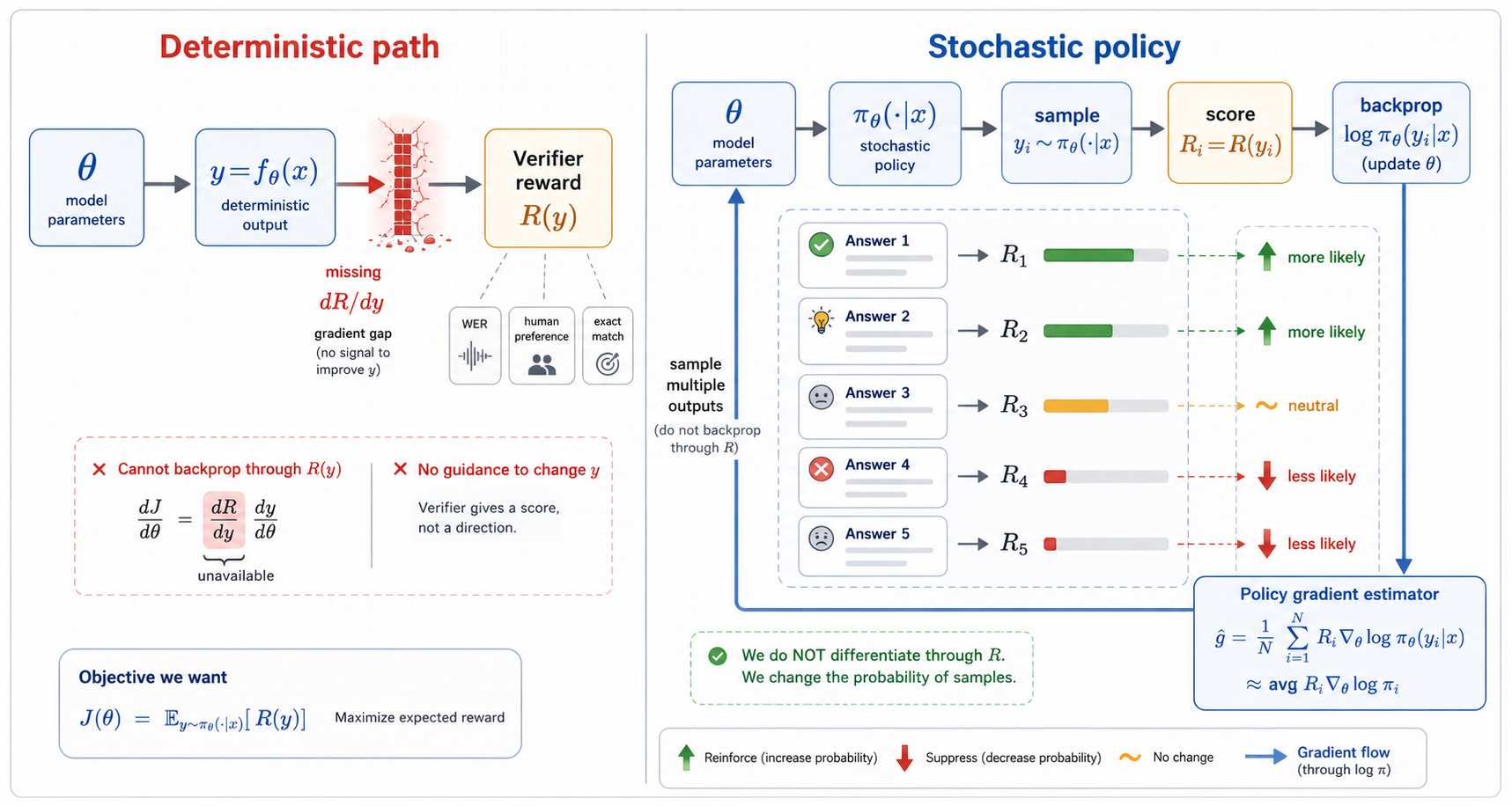
Plenty of the rewards we actually care about simply don’t give us this gradient. A verifier reports whether an answer is correct. A human can prefer answer A to answer B. An ASR system emits a transcript, and WER comes out of an edit-distance computation. For a concrete sample, all of these can produce a label or score. What they do not produce is a useful gradient with respect to the model output.

So we hit a wall:

The reward tells us whether the output was good. It never tells us how to nudge the output to make it better.

Deterministic policy gradient methods have one answer to this: learn a critic, a Q-function that estimates long-term value.

$$Q^\pi(s,a) = \mathbb{E}_\pi \left[ \sum_{t=0}^{\infty} \gamma^t r_t \mid s_0=s, a_0=a \right]$$

If $Q(s,a)$ is differentiable in the action $a$, a deterministic actor can ride its gradient uphill:

$$\nabla_\theta J \approx \nabla_a Q(s,a) \big|_{a=\mu_\theta(s)} \cdot \nabla_\theta \mu_\theta(s)$$

In effect, the critic supplies the missing direction: it tells us which way the action should move.

But for high-dimensional generation with sparse, black-box, verifier-style rewards, training a reliable critic is hard and often unstable. There’s a second route that sidesteps the whole problem. Instead of asking how the output should move, ask a different question entirely: which of the outputs I already sampled should become more likely?

That’s the stochastic strategy.

---

4. The Stochastic Strategy: Optimize the Distribution

A stochastic policy doesn’t commit to a single output. It defines a distribution:

$$y \sim \pi_\theta(\cdot \mid x)$$

Two notations that are easy to blur together:

• $\pi_\theta(\cdot \mid x)$ is the entire output distribution given $x$.
• $\pi_\theta(y \mid x)$ is the probability (or density) of one specific output $y$.

The objective changes shape. We’re no longer maximizing the score of a single deterministic output. We’re maximizing expected reward over the distribution:

$$J(\theta) = \mathbb{E}_{y\sim\pi_\theta(\cdot \mid x)} \left[ R(y) \right]$$

Written as an integral:

$$J(\theta) = \int \pi_\theta(y \mid x) R(y) \,dy$$

and for discrete outputs, the integral is just a sum:

$$J(\theta) = \sum_y \pi_\theta(y \mid x)R(y)$$

This is nothing more exotic than a probability-weighted average reward. We want the model to move its probability mass toward the high-reward outputs.

And here’s the inversion that makes everything downstream work:

We don’t need to know how to edit a specific output to raise its reward.

We only need to know how to reshape the model so that high-reward sampled outputs become more likely.

---

5. SFT First: Increasing the Probability of a Gold Answer

Before deriving policy gradient, let’s re-anchor on SFT, because the two turn out to be siblings.

In SFT the dataset hands us a gold answer:

$$y_{\text{gt}}$$

and the objective is maximum likelihood:

$$\max_\theta \log \pi_\theta(y_{\text{gt}} \mid x)$$

which is the same as minimizing cross entropy:

$$\mathcal{L}_{\text{SFT}} = - \log \pi_\theta(y_{\text{gt}} \mid x)$$

For an autoregressive LLM, the sequence probability factorizes token by token:

$$\pi_\theta(y_{\text{gt}} \mid x) = \prod_{t=1}^{T} \pi_\theta(y_t \mid x, y_{<t})$$

and taking the log turns that product into a sum:

$$\log \pi_\theta(y_{\text{gt}} \mid x) = \sum_{t=1}^{T} \log \pi_\theta(y_t \mid x, y_{<t})$$

So SFT, stripped to one line, says:

Given a trusted answer, raise the log probability of the token path that produces it.

Hold onto that shape. Policy gradient is going to look almost identical, with one decisive change: the answer is sampled by the model itself, and its weight comes from reward.

---

6. Why We Need the Log Trick

We want the gradient of the objective:

$$\nabla_\theta J(\theta)$$

Start from the integral form:

$$J(\theta) = \int \pi_\theta(y \mid x)R(y) \,dy$$

and differentiate:

$$\nabla_\theta J(\theta) = \int \nabla_\theta \pi_\theta(y \mid x) R(y) \,dy$$

This is correct, but it’s stuck. We can’t estimate it by sampling from $\pi_\theta$ yet, and sampling is the only thing we can actually do. Monte Carlo estimation needs the integrand to wear a particular costume:

$$\int \pi_\theta(y \mid x) f(y) \,dy = \mathbb{E}_{y\sim\pi_\theta} [f(y)]$$

because then we can draw samples

$$y_1,\dots,y_N \sim \pi_\theta(\cdot \mid x)$$

and approximate the expectation by averaging:

$$\mathbb{E}[f(y)] \approx \frac{1}{N} \sum_{i=1}^{N} f(y_i)$$

The snag is that our gradient contains

$$\nabla_\theta \pi_\theta(y \mid x)$$

not the bare

$$\pi_\theta(y \mid x)$$

that the Monte Carlo form requires out front. We need to coax $\pi_\theta$ back into that leading position.

Enter the score-function trick. It starts from the ordinary derivative of a log:

$$\nabla_\theta \log \pi_\theta(y \mid x) = \frac{1}{\pi_\theta(y \mid x)} \nabla_\theta \pi_\theta(y \mid x)$$

Rearranged, that’s exactly the substitution we need:

$$\nabla_\theta \pi_\theta(y \mid x) = \pi_\theta(y \mid x) \nabla_\theta \log \pi_\theta(y \mid x)$$

Drop it back into the gradient:

$$\nabla_\theta J(\theta) = \int \pi_\theta(y \mid x) R(y) \nabla_\theta \log \pi_\theta(y \mid x) \,dy$$

and now the integrand is in Monte Carlo costume,

$$\int \pi_\theta(y \mid x) f(y)\,dy, \qquad f(y) = R(y) \nabla_\theta \log \pi_\theta(y \mid x)$$

so the gradient is just an expectation:

$$\nabla_\theta J(\theta) = \mathbb{E}_{y\sim\pi_\theta(\cdot \mid x)} \left[ R(y) \nabla_\theta \log \pi_\theta(y \mid x) \right]$$

This is the REINFORCE estimator, also called the score-function or likelihood-ratio estimator.

One thing to keep straight through all of this: the reward is a constant with respect to $\theta$. It’s a black box that hands back a number, nothing more. Differentiable pieces like a KL penalty don’t live inside $R$; they’re tacked on separately as their own loss term.

And notice why the log showed up. It wasn’t a clever nod to SFT. It appeared because we had to rewrite

$$\nabla_\theta \pi_\theta \qquad\text{as}\qquad \pi_\theta \nabla_\theta \log \pi_\theta$$

so that the gradient could be estimated by sampling from $\pi_\theta$. The resemblance to SFT is a consequence, not the motivation, which is exactly what makes it satisfying.

---

7. Monte Carlo: Engineering the Law of Large Numbers

The exact expectation is hopeless to compute, because the output space is astronomically large. This is the practical pain that the clean notation quietly papers over.

In the integral, $y$ ranges over every possible output:

$$\int \pi_\theta(y\mid x) R(y) \nabla_\theta \log \pi_\theta(y\mid x) \,dy$$

Mathematically that’s well-defined. Computationally it’s a fantasy. We can’t loop over every completion an LLM might produce, score each one, take each log-prob gradient, and sum it all up.

So we don’t. We sample:

$$y_1,\dots,y_N \sim \pi_\theta(\cdot \mid x)$$

and estimate:

$$\nabla_\theta J(\theta) \approx \frac{1}{N} \sum_{i=1}^{N} R(y_i) \nabla_\theta \log \pi_\theta(y_i \mid x)$$

That’s Monte Carlo estimation, and the engine underneath it is the law of large numbers:

$$\frac{1}{N} \sum_{i=1}^{N} f(y_i) \rightarrow \mathbb{E}[f(y)] \quad\text{as } N\to\infty$$

This is the moment the symbols turn into computation. The abstract variable $y$ becomes a handful of concrete samples $y_i$, and every term in the sum is something we can actually evaluate:

Symbol	Meaning	Can we compute it directly?
$y$	A variable over the entire output space	No: too many possible outputs to enumerate.
$y_i$	One sampled output from the current model	Yes: it’s a concrete sequence.
$R(y_i)$	Reward of that sampled output	Yes: the verifier returns a scalar.
$\nabla_\theta \log \pi_\theta(y_i\mid x)$	Gradient of the sample’s log probability	Yes: ordinary backprop, exactly like SFT.

The name “Monte Carlo” is just a label for this practice: the samples are model outputs, the function is reward times score, and their average estimates the gradient. This is where trial and error becomes mathematics, and it lines up perfectly with the classroom. The student tries several answers, the teacher scores them, and the update rule reads:

Answers that scored higher should become more likely next time.

---

8. From Gradient Estimator to Loss

In practice we don’t hand-code gradients. We write a loss and let backprop do the rest.

For a single sampled output $y_i$, the simplest policy-gradient loss is:

$$\mathcal{L}_{\text{PG}} = - R(y_i) \log \pi_\theta(y_i \mid x)$$

In real systems, though, we almost always swap the raw reward for an advantage:

$$\mathcal{L}_{\text{PG}} = - A(y_i) \log \pi_\theta(y_i \mid x)$$

The advantage answers a sharper question: was this output better than some baseline?

$$A(y_i) = R(y_i)-b$$

Why are we allowed to subtract a baseline at all? Because as long as $b$ doesn’t depend on the sampled action, it vanishes in expectation:

$$\mathbb{E}_{y\sim\pi_\theta} \left[ b\nabla_\theta\log\pi_\theta(y\mid x) \right] = b\nabla_\theta \int \pi_\theta(y\mid x)\,dy = b\nabla_\theta 1 = 0$$

So the baseline leaves the expected gradient untouched; it only cuts the variance. This is the first place engineering quietly enters the story: the estimator is unbiased but noisy, so we reshape the reward into a steadier learning signal without biasing it.

The sign of the advantage is what drives learning. When

$$A(y_i)>0,$$

minimizing the loss pushes the log probability of $y_i$ up. When

$$A(y_i)<0,$$

it pushes that log probability down. Good attempts get reinforced; bad ones get suppressed.

And this is precisely why policy gradient feels like a weighted version of SFT. Put them next to each other:

$$\mathcal{L}_{\text{SFT}} = - \log \pi_\theta(y_{\text{gt}}\mid x) \qquad\qquad \mathcal{L}_{\text{PG}} = - A(y) \log \pi_\theta(y\mid x)$$

The difference is not cosmetic. In SFT the answer comes from the dataset and is trusted as gold. In policy gradient the answer is sampled by the current model and weighted by feedback. Same skeleton, completely different source of truth.

The same contrast, with GRPO added as the natural next step:

Method	Where the answer comes from	What is optimized	Mental model
SFT	A gold answer from the dataset	$-\log \pi_\theta(y_{\text{gt}}\mid x)$	Imitate the answer key.
Policy gradient	A sample from the current model	$-A(y)\log \pi_\theta(y\mid x)$	Reinforce the better attempts.
GRPO	A group of samples from the current model	$-A_i\log \pi_\theta(y_i\mid x)$, with group-relative $A_i$	Reward-weighted SFT, weights normalized within the group.

For an autoregressive LLM, one detail is worth spelling out: the sequence-level advantage multiplies the entire sum of token log-probabilities:

$$\mathcal{L}_{\text{PG}} = - A(y_i) \sum_{t=1}^{T} \log \pi_\theta(y_{i,t}\mid x,y_{i,<t})$$

Every token in the sampled answer inherits the same sequence-level feedback. As credit assignment goes, that’s blunt, but the bluntness is exactly what keeps the method simple enough to scale.

So the classroom metaphor sharpens into something precise:

• SFT is memorizing the teacher’s answer key.
• Policy gradient is trying several answers, collecting scores, and reinforcing the strategies that worked.

---

9. GRPO: Group Relative Policy Optimization

GRPO stands for Group Relative Policy Optimization, and the core idea is almost embarrassingly simple.

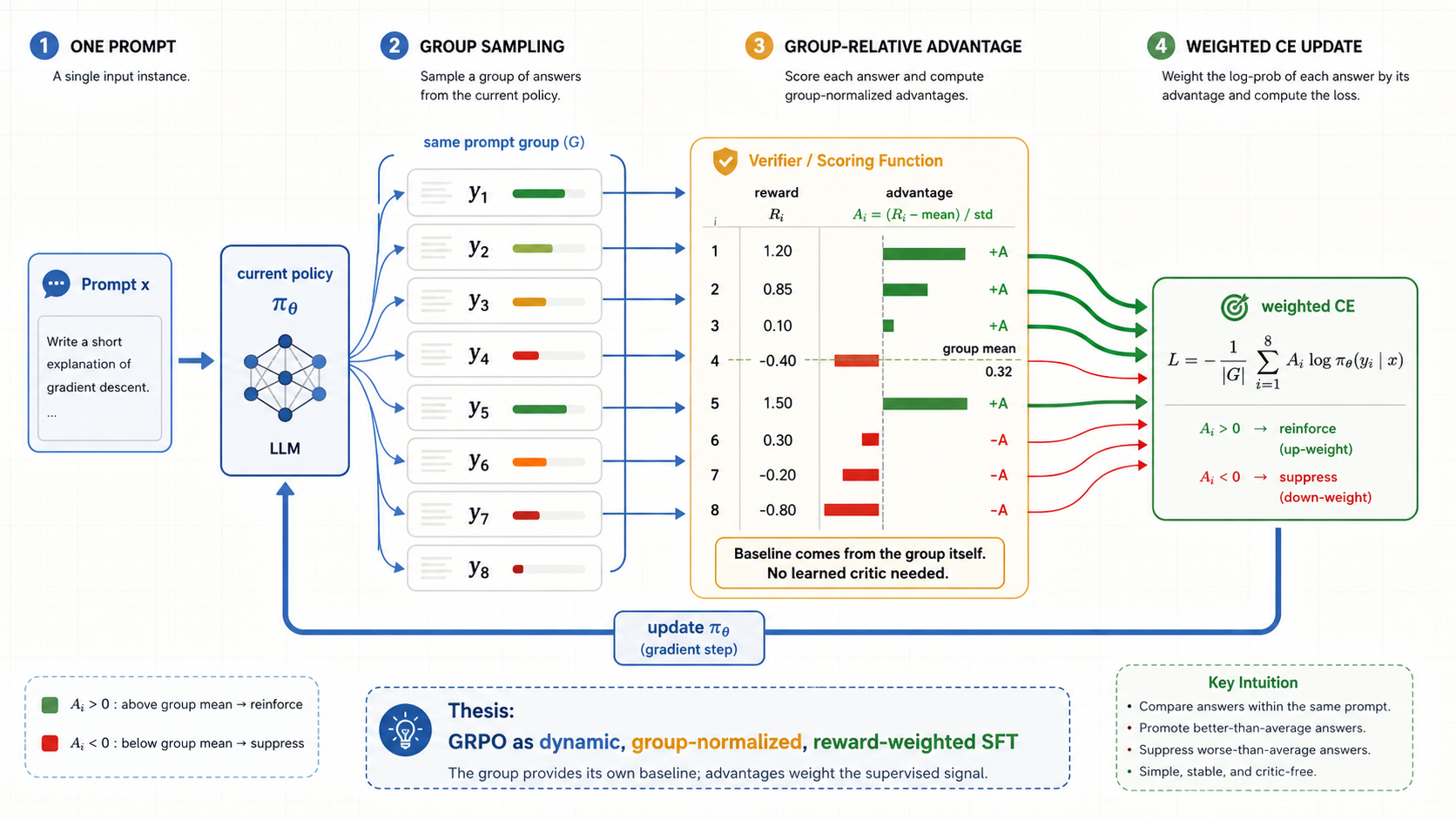
For a single prompt $x$, sample a whole group of outputs at once:

$$y_1,\dots,y_G \sim \pi_\theta(\cdot \mid x)$$

score each one:

$$R_1,\dots,R_G$$

and then build a group-relative advantage by standardizing those scores against each other:

$$A_i = \frac{ R_i-\mathrm{mean}(R_1,\dots,R_G) }{ \mathrm{std}(R_1,\dots,R_G) }$$

This converts raw rewards into something closer to class rank. A sample doesn’t have to be perfect, or even objectively good. It just has to land above the group average to get reinforced. That’s the whole trick: no separately trained critic, no learned value baseline. The other samples in the group are the baseline.

From there it’s the same weighted-logprob loss we already have:

$$\mathcal{L}_{\text{GRPO}} \sim - A_i \log \pi_\theta(y_i\mid x)$$

Production GRPO bolts on a few stabilizers (old-policy probability ratios, clipping, KL regularization against a reference model, reward normalization), but none of them disturb the mental model:

Sample several answers. Score them. Standardize the scores within the group. Push up the probability of the above-average samples and push down the below-average ones.

Which is why GRPO is fairly read as dynamic weighted SFT: the weights aren’t fixed in a dataset, they’re constructed online from group-relative reward.

---

10. Why KL Regularization Appears

Reward functions are imperfect, and a model under optimization pressure is very good at finding the cracks.

Optimize the reward and nothing else, and the model will happily exploit the verifier rather than the task. A text model discovers strange formatting tricks. An audio model learns to be easy for an ASR verifier to transcribe while sounding unnatural to a human ear. A code model overfits the unit tests and ships brittle solutions. Reward hacking, in every flavor.

The standard guardrail is to keep the model tethered to a reference model

$$\pi_{\text{ref}}$$

with a KL penalty:

$$D_{\mathrm{KL}} \left( \pi_\theta(\cdot \mid x) \;\|\; \pi_{\text{ref}}(\cdot \mid x) \right)$$

The two forces balance against each other. Reward pulls the model toward outputs that score better; KL holds it near a distribution we already trust. It isn’t mathematical decoration; it’s the practical brake that keeps reward optimization from driving off a cliff.

---

11. When Should You Reach for SFT, DPO, PPO, or GRPO?

None of this is an argument that GRPO is the best tool. The point is narrower and more useful: GRPO solves a particular kind of problem, and knowing which problem you have tells you which tool to grab.

If you have gold answers, SFT is the simplest thing that works:

$$\mathcal{L}_{\text{SFT}} = - \log \pi_\theta(y_{\text{gt}}\mid x)$$

If you have a fixed set of preference pairs, methods like DPO are the natural fit. However those pairs were collected, the update treats them as an offline dataset: no fresh on-policy sampling each step, just a differentiable objective over the policy and a reference.

If you have an external reward or verifier that can score the current model’s outputs but can’t hand back a useful gradient, policy-gradient methods like PPO and GRPO come into their own.

If your reward and your generation path are both fully differentiable and the gradient is trustworthy, skip the estimator entirely and backpropagate directly; it usually has lower variance than a score-function estimate. If a reward can be written as a smooth differentiable loss, there’s no reason to launder it through REINFORCE.

As a quick decision table:

What you have	Typical method	Why
Gold answers	SFT	The answer key is known: just maximize its likelihood.
Fixed / pre-collected preference pairs	DPO-style preference optimization	The comparison data already exists offline.
Online black-box rewards	PPO / GRPO-style policy gradient	The verifier scores samples but offers no usable gradient.
Differentiable rewards and differentiable generation	Direct reward loss	If the gradient is trustworthy, use it instead of estimating it.

The headline: GRPO isn’t valuable because rewards are computable. It’s valuable because so many of the rewards we actually want are not reliably differentiable.

---

12. Beyond LLMs: Why Probability Matters

For a standard sampled LLM, the policy distribution is handed to you for free. The model emits token probabilities, you sample from them, and you can read off

$$\log \pi_\theta(y\mid x)$$

for whatever sequence you sampled. Everything above just works.

For other generative models, that’s not guaranteed.

Take a flow-matching generator. It may begin from sampled base noise and then follow a deterministic trajectory through a learned velocity field. The subtle catch is that, unlike an LLM, it may never expose a trainable log probability, neither for the intermediate steps nor for the final trajectory.

And the moment that term goes missing, the policy-gradient story falls apart:

$$R(y) \nabla_\theta \log \pi_\theta(y\mid x)$$

needs a probability model with tractable log probabilities. Strip out $\log\pi_\theta$ and the score-function update has nothing left to backpropagate through.

This is why some non-LLM systems that want GRPO-style training have to make their generation probabilistic first, or otherwise manufacture the log probabilities that policy gradient depends on. In flow-matching TTS, for example, the model can be set up to sample from an output distribution instead of emitting a single deterministic velocity. Once the trajectories carry log probabilities, policy-gradient training is back on the table.

That’s the bridge to systems like F5-R-style TTS: if you want to optimize black-box rewards such as WER or speaker similarity with policy gradient, the generator has to supply not just samples but the log probabilities of those samples. No log-probs, no policy gradient.

---

13. The Whole Picture

Here’s the entire chain in one place.

We want to maximize expected reward:

$$J(\theta) = \mathbb{E}_{y\sim\pi_\theta} [R(y)]$$

Write it as an integral:

$$J(\theta) = \int \pi_\theta(y\mid x)R(y) \,dy$$

Take the gradient:

$$\nabla_\theta J = \int \nabla_\theta \pi_\theta(y\mid x) R(y) \,dy$$

Apply the score-function trick:

$$\nabla_\theta \pi_\theta(y\mid x) = \pi_\theta(y\mid x) \nabla_\theta \log \pi_\theta(y\mid x)$$

which turns the gradient into an expectation:

$$\nabla_\theta J = \mathbb{E}_{y\sim\pi_\theta} \left[ R(y) \nabla_\theta \log \pi_\theta(y\mid x) \right]$$

estimate it with Monte Carlo:

$$\nabla_\theta J \approx \frac{1}{N} \sum_{i=1}^{N} R(y_i) \nabla_\theta \log \pi_\theta(y_i\mid x)$$

implement it as weighted log-prob training:

$$\mathcal{L} = - A(y_i) \log \pi_\theta(y_i\mid x)$$

and, for GRPO, build the weights by comparing samples within a group:

$$A_i = \frac{ R_i-\mathrm{mean}(R_1,\dots,R_G) }{ \mathrm{std}(R_1,\dots,R_G) }$$

Which leaves the mental model right where we started, now fully earned:

SFT raises the probability of gold answers.

Policy gradient raises or lowers the probability of sampled answers according to advantage.

GRPO constructs those weights by comparing samples within the same group.

That’s the missing bridge between classical reinforcement learning and modern LLM post-training, and it’s why GRPO, for all its production machinery, is best understood as dynamic, group-normalized, reward-weighted SFT on the model’s own samples.